From my experience in solving machine learning problem, about 50% of the problems I've faced are classification problems, and a sizable percentage of these classification problems are imbalanced.

An imbalanced problem is a classification problem in which one of the target classes dominates the other. For example, in a binary classification problem with two classes - 1 and 0, 80% of the data points have a target of class 1. This means as the machine learning engineer working on this, you will have much more information on class 1 as compared to class 0. To check if a given dataset is imbalanced, you can easily use the value_count function on the target column.

Handling imbalanced datasets

There are many well-documented methods of handling imbalanced datasets, but the approach that will be discussed in this article which is rare has helped me immensely in machine learning competitions (binary classification tasks). Whilst one of the more popular methods include Oversampling, Undersampling and Parameter tuning [tuning parameters like scale_pos_weight and class_weights in models like xgboost, catboost and lightgbm], the method of interest is tuning the classification threshold.

This approach involves training a simple model on the dataset and changing the probability threshold. Usually, normal binary classification models use a probability threshold of 0.5, which means predictions that have predicted probability < 0.5, will be predicted as class 0, while those with predicted probability >= 0.5 will be predicted as class 1. This approach involves reducing or increasing the threshold from 0.5.

At this point, a valid question would be to ask How do you know/determine the new threshold to use?

It is quite simple! Just tune the threshold on the validation data and see which produces better performance on the metric you are using (f1_score is commonly used for imbalanced datasets). This process comes with the risk of overfitting. As such, be careful. I admit that at this point, this concept might still seem confusing. Not to worry, the coding solution in the next session should shed more light.

Coding solution

The dataset used is obtained from the Landslide Prevention and Innovation Challenge on zindi.africa .

The main aim of the challenge is to identify if a landslide occurred or not and the evaluation metric for this challenge is the f1_score. A train and test datasets are provided. Download the train and test data, and ensure that they are in the same folder as your notebook.

The full notebook can be found here .

Prerequisites

• A fundamental understanzding of the workings of Machine Learning models.

• Experience with Scikit-learn, pandas and matplotlib.

Step 1: Importing the necessary libraries

To begin, you will import the dependencies needed to prepare your data for preprocessing and create your model.

import numpy as np
import pandas as pd
import seaborn as sns
from sklearn.model_selection import train_test_split
from sklearn.ensemble import RandomForestClassifier
from sklearn.metrics import f1_score
import matplotlib.pyplot as plt

Step 2: Loading and exploring the dataset

train=pd.read_csv("Train.csv",index_col=0)
test=pd.read_csv("Test.csv",index_col=0)

Next, you will remove the target column from your train data and do a countplot to visualize the value_count of each class.

target=train["Label"]
train.drop("Label",axis=1,inplace=True)

sns.countplot(target)

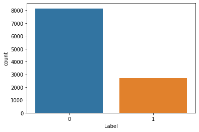
As you can see, the 0 class has a count of about three times that of the 1 class.

print(train.shape)

The output is as follows;

(10864, 225)

There are 225 columns here which is quite large and you can do a lot of data cleaning and feature combination to improve the model performance but that is not the main aim of this article.

You must split the train data into X and validation sets.

X,val,y,y_val=train_test_split(train,target,test_size=0.2,random_state=0)

Step 3: Building the model and making predictions.

model=RandomForestClassifier(verbose=2,random_state=0,n_estimators=1000)

model.fit(X,y)

Predicting the probability;

y_predicted_proba=pd.Series(model.predict_proba(val)[:,1])

Predicting on the validation dataset;

You should create a function that accepts the probability and threshold as parameters, the function should convert the probability to a class based on the threshold parameter.

def tune_treshold(proba,threshold):
  if proba>threshold:
    return 1
  else:
    return 0

You will then make predictions for each threshold in the range of 0 and 1, and append the f1_score to a list.

threshold_range=np.arange(0,1,0.01)
f1_scores=[]
for i in threshold_range:
  tuned_predictions=y_predicted_proba.apply(tune_treshold,args=(i,))
  f1_scores.append(f1_score(tuned_predictions,y_val))

You then create a simple plot of the f1_scores to the probability thresholds, so you can see the threshold better .

plt.plot(threshold_range,f1_scores)

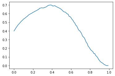
You can zoom the plot in, by reducing the range and the step so you can see the threshold better.

threshold_range=np.arange(0.35,0.4,0.0001)
f1_scores=[]
for i in threshold_range:
  tuned_predictions=y_predicted_proba.apply(tune_treshold,args=(i,))
  f1_scores.append(f1_score(tuned_predictions,y_val))

plt.plot(threshold_range,f1_scores)

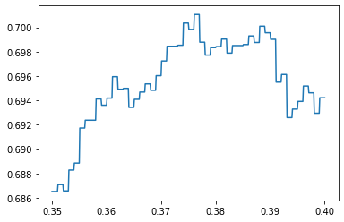
best_threshold=0.375

The best threshold to use from the plot is 0.375.

The validation score:

print(f"Your validation f1_score is {f1_score(y_predicted_proba.apply(tune_treshold,args=(best_treshold,)),y_val)}")

Your validation f1_score is 0.699825479930192

Finally, Create a submission file (predicting the probabilities) and use the probability threshold to predict the classes.

sub=pd.DataFrame({"Sample_ID":test.index,"Label":model.predict_proba(test)[:,1]}).set_index("Sample_ID")
sub["Label"]=sub["Label"].apply(tune_treshold,args=(best_treshold,))

sub.to_csv("sub_landslide.csv")

The full notebook can be found here.

Results on the leaderboard:

Using the same model with the normal threshold (0.5) gave a leaderboard score of 0.675 (position 80 as at the time this article is being written) and tuning the probability threshold gave me a leaderboard score of 0.733 (position 55 as at the time this article is being written).

Many improvements can be done to the model and data to improve the f1_score.

Conclusion

It is worthy of note that there are many approaches you can try when handling an imbalanced dataset and this is just one of them! You should try other approaches also and see which gives you better results.